👨‍🏫 Outline of Lecture 1

Capital Allocation

1. Capital Allocation: The “Top Down” Approach
2. Three-step process of portfolio construction
3. Capital allocation between risky and risk-free assets
4. The CAL line

Portfolio Construction: The “Top Down” Approach

• Capital Allocation Decision
  • Allocation of portfolio between a risk-free asset and risky assets
• Asset Allocation Decision
  • Distribution of risky investments across broad asset classes (e.g. bonds, stocks, currencies, etc.)
• Security Selection Decision
  • Choice of individual securities within each (risky) asset class

Capital Allocation Across Risky and Risk-Free Portfolios

The simplest way to control risk is to manipulate the fraction of the portfolio invested in risk-free assets versus the portion invested in the risky assets

Basic Asset Allocation Example

Total market value	$300,000
Risk-free money market fund	$90,000
Equities	$113,400
Bonds (long-term)	$96,600
Total risky assets	$210,000

Percentage of risky portfolio in Equities and Bonds:

$$W_{E} = \frac{\$113,400}{\$210,000} = 0.54=54\%$$ $$W_{B} = \frac{\$96,000}{\$210,000} = 0.46=46\%$$

Let

• $y$ = Weight of the risky portfolio, P, in the complete portfolio
• $(1-y)$ = Weight of risk-free assets

$$y = \frac{\$210,000}{\$300,000} = 70\%$$ $$1 - y = \frac{\$90,000}{\$300,000} = 30\%$$

Percentage of complete portfolio in Equities and Bonds:

$$E:\frac{\$113,400}{\$300,000} = 37.8\%$$ $$B:\frac{\$96,600}{\$300,000} = 32.2\%$$

The Risk-Free Asset

• Only the government can issue default-free securities
  • A security is risk-free in real terms only if its price is indexed and its maturity is equal to the investor’s holding period
• T-bills viewed as “the” risk-free asset
• Money market funds also considered risk-free in practice

Capital Allocation Decision: One Risky and One Risk-Free Asset

Notation	Meaning
$y$	= Proportion of capital invested in risky asset
$1 - y$	= Proportion of capital invested in risk-free asset
$r_P$	= rate of return on risky asset
$E(r_P)$	= expected rate of return on risky asset
$σ_P$	= standard deviation of return on risky asset
$r_F$	= rate of return on risk-free asset
$E(r_P) - r_F$	= risk premium on the risky asset
$r_C$	= rate of return on the complete portfolio

$$\begin{aligned} r_C &= \text{Rate of return of complete portfolio} \\ &= yr_P+(1-y)r_F \quad ①\\ \end{aligned}$$

The second line (formula ①) is important because it shows us how to think of the return of a portfolio. Specifically, we think of the Complete portfolio as being a mixture of a risk-free asset and a risky asset. In probability, we calculate mixtures using weighted averages, so the return of our complete portfolio will be a weighted average of the return on the risky asset and the risk-free asset. Writing this as a formula, we get the equation that Bruce put in the slides - that the rate of return of the complete portfolio is $r_C=yr_P+(1-y)r_F$.

If you aren’t familiar with weighted averages, this step may not make sense to you. That’s fine - just try to remember the formula.

$$\begin{aligned} E(r_C) &= \text{Exp return of complete port} \\ &= E[yr_P + (1-y)r_F] \quad ② \\ &= yE(r_P) + (1-y)E(r_F) \quad ③ \\ &= yE(r_P) + (1-y)r_F \quad ④ \\ &= r_F + y[E(r_P)-r_F] \quad ⑤ \\ \end{aligned}$$

I suspect you can afford to gloss over some of the slides of math later on in this lecture, but I think this slide is worth going into a little more deeply. Here are the key steps:

Formula 2

This step works because of formula ①, discussed about two paragraphs above. Specifically, it works because the complete portfolio is just a mixture of a risky asset and a risk-free asset.

Formula 3

This follows from a math fact from probability. It’s a deep math fact that underlies this entire topic. I discuss it at the bottom of the page entitled 🔎 Where did our two formulas come from?.

Formula 4

This step is intuitive. What is the expected value of the risk free rate? Well, we know exactly what the return on the risk-free asset will be. That’s what it means for the asset to be risk free: we know in advance exactly what the return will be. Therefore, $r_F$ is not random. We know the true value, and our expected value is exactly equal to the true value. Mathematically, $E(r_F)=r_F$.

Formula 5

This is just rearranging the terms from formula ④ using algebra. Algebra isn’t a focus of this course, so don’t worry if you have trouble seeing how ④ and ⑤ are equivalent.

While the 5 steps above are helpful, the main point is the final equation, which Bruce explains as follows:

The formula above shows that $r_F$, the risk free rate, is a base rate of return on any portfolio:

Expected return on the complete portfolio = base rate (risk-free rate) + the risk premium on the risky asset weighted by the proportion of the total portfolio invested in the risky asset

$E(r_P) - r_F > 0$ assuming investors are risk-averse

Calculating the Standard Deviation of the Portfolio Return

Recall that, if X and Y are independent random variables and a and b and constants:

$Var(aX + bY) = a^{2}Var(X) + b^{2}Var(Y)$
Here, $X = r_P$ and $Y = r_f$

So,

$$\begin{aligned} Var\left(r_c \right) &= Var[yr_P + (1 - y)r_f] \\ &= y^{2}Var\left(r_P \right) + (1 - y)^{2}Var\left(r_f \right) \\ &= y^{2}Var\left(r_P \right) + 0 \\ &= y^{2}Var\left(r_P \right) \\ \end{aligned}$$

Taking the square root of both sides and remembering that $\sqrt{Var}=σ$

$$σ_c = y σ_P$$

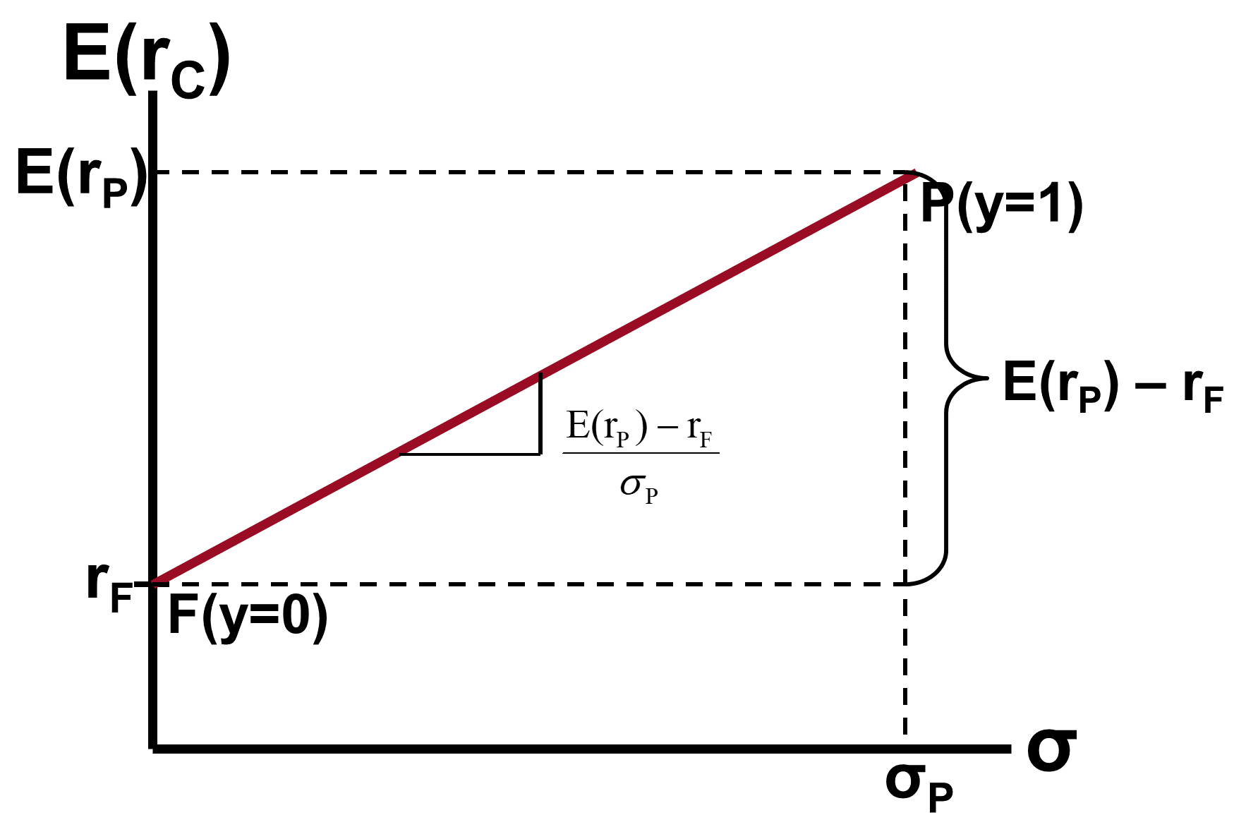
Equation for the CAL

$$σ_c = y \times σ_P$$ $$y = \frac{σ_c}{σ_P}\$$ $$E(r_c ) = r_f\ + \frac{σ_c}{σ_P}[E\left(r_P \right)-\ r_f]$$ $$E\left(r_c \right) = \ r_f\ + \frac{[E\left(r_P \right)-\ r_f]}{σ_P}σ_c$$

$\frac{[E\left(r_P \right)-\ r_f]}{σ_P}$ is known as the Sharpe ratio or Reward-to-variability ratio.

Let $σ_P = 20\%$ and $y = 50\%$. Therefore

$$σ_c = y \times σ_P = 50\%\times 20\% = .1 = 10\%$$ $$r_f = 5\%$$
$$E\left(r_P \right) = 10\% = \ .1$$ $$\text{Sharpe ratio} = \frac{E\left(r_P \right) - r_f}{σ_P}\ = \frac{.1 - .05}{.2} = \ .25$$ $$\begin{aligned} E\left(r_c \right) &= \ r_f\ + \frac{[E\left(r_P \right)-\ r_f]}{σ_P}σ_c \\ &= \ .05 + \ .25(.1) \\ &= \ .075 \\ &= 7.5\% \\ \end{aligned}$$

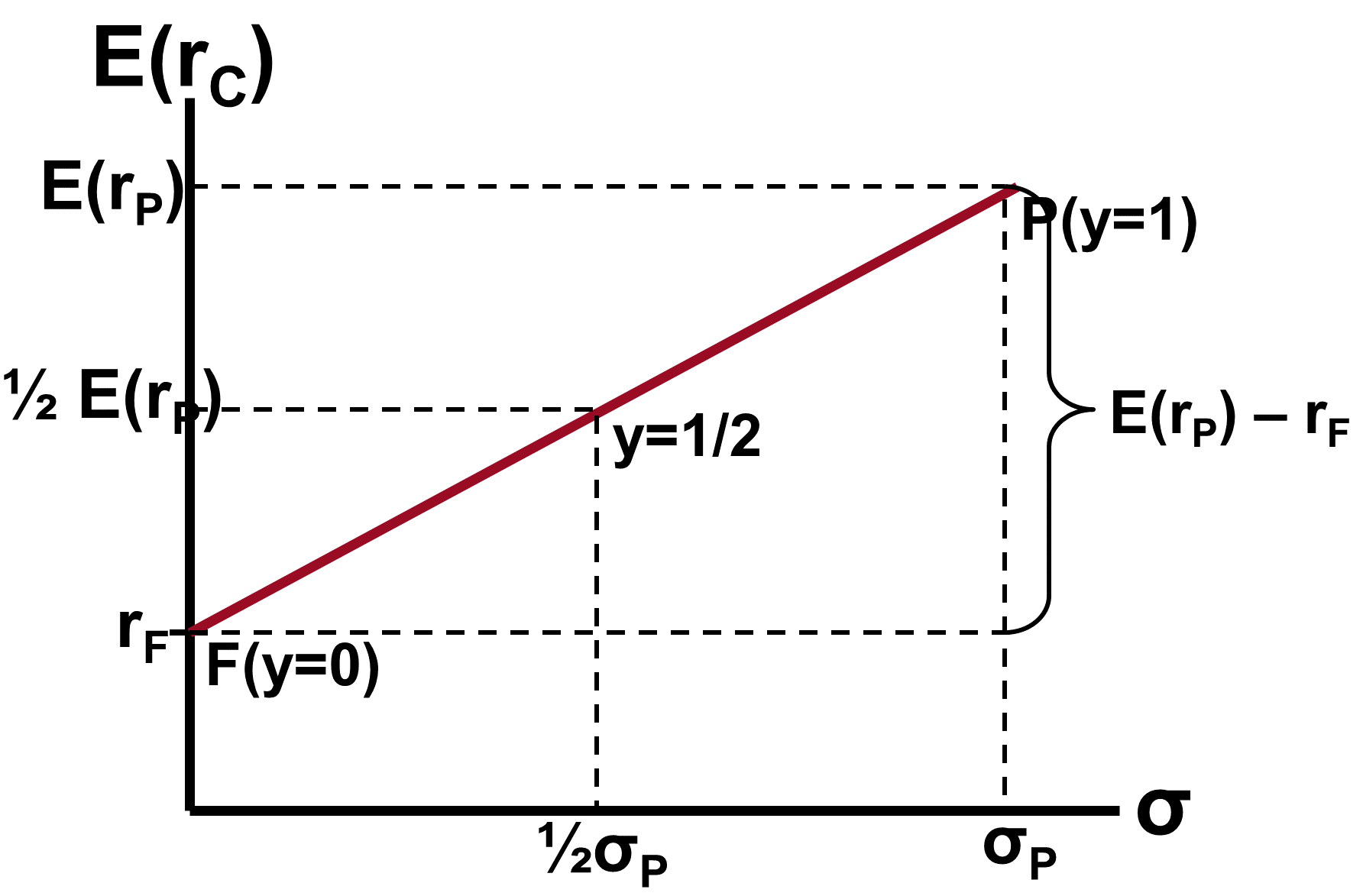
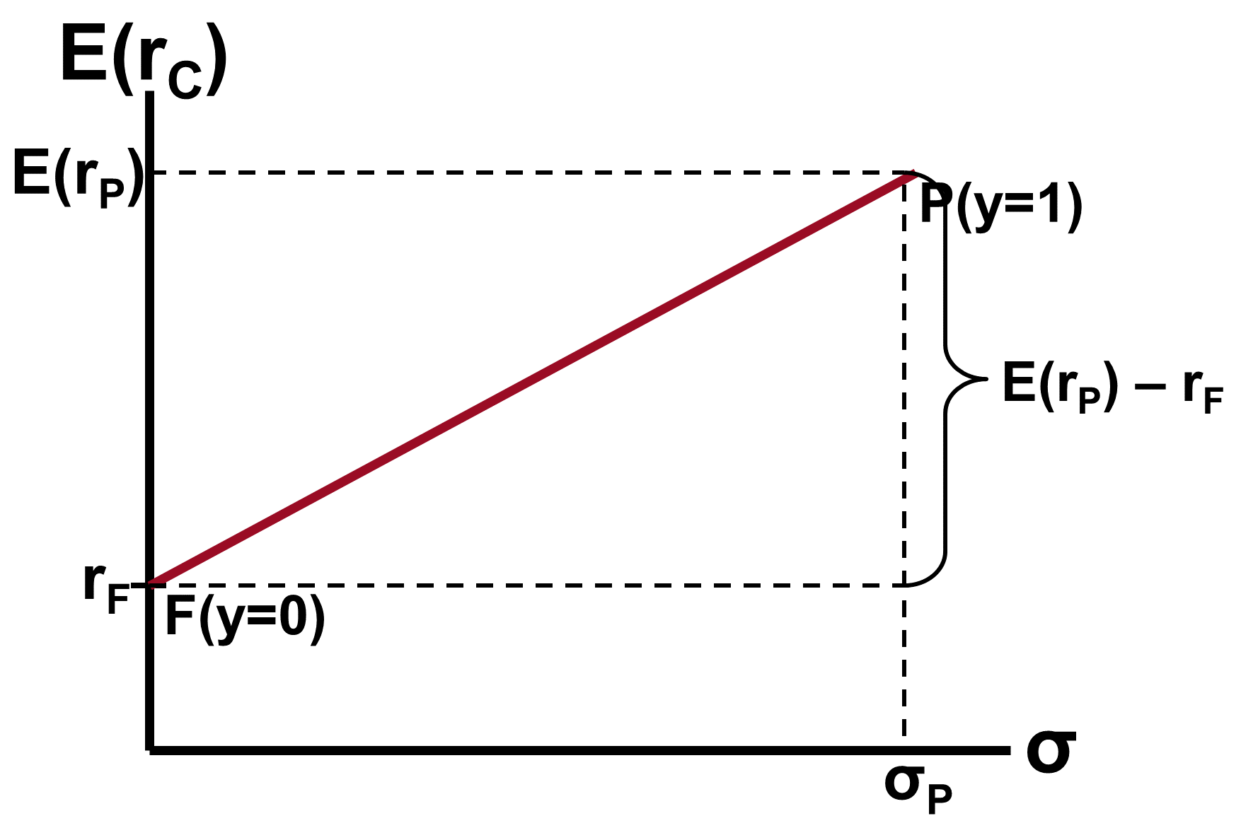
The Capital Allocation Line (CAL)

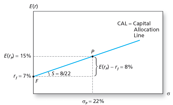
One Risky Asset and a Risk-Free Asset: Example

$$r_f = 7\%$$ $$E(r_P) = 15\%$$ $$σ_{rf} = 0\%$$ $$σ_P = 22\%$$

The expected return on the complete portfolio:

$$E(r_c) = 7 + y(15 - 7)$$

The risk of the complete portfolio:

$$σ_c = yσ_P = 22y$$

Rearranging:

$$y = \frac{σ_c}{σ_P}$$

Substitute into CAL equation:

$$E(r_c) = r_f\ + \frac{σ_c}{σ_P}[E(r_P) - r_f]$$ $$Slope = \frac{E(r_P) - r_f}{σ_P} = \frac{8}{22}$$

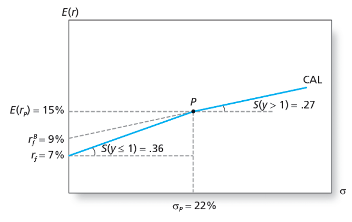
The Investment Opportunity Set

Portfolios of One Risky Asset and a Risk-Free Asset

• Capital allocation line with leverage
  • Lend at $r_f= 7\%$ and borrow at $r_f= 9\%$
    • Lending range slope = $8/22 = 0.36$
      • “Lending range” is the portion of the CAL where y is less than 1, so the investor is investing in the risk-free asset. By investing in the risk free asset, they are “lending” money.
    • Borrowing range slope = $6/22 = 0.27$
      • “Borrowing range” is the portion of the CAL where y is greater than 1. The portion of the investor’s wealth invested in the risky asset is $1-y$. If $y>1$, then $(1-y)< 0$, so the investor has a negative investment in the risk free asset. They are essentially attempting to “borrow” money. Because they they might not repay the loan, they can’t borrow at the risk-free rate, and this reduces their Expected return. This causes the CAL to have a lower slope in the borrowing range.
  • CAL kinks at $y=1$, where $r_C=r_P$.

The Opportunity Set with Differential Borrowing and Lending Rates

Example:

Two Assets:

$$E(r_1)=8\%, σ 1= 12\%$$ $$E(r_2)=13\%, σ 2= 20\%$$