❔ CAPM FAQs

🙋 The CAPM equation is similar to the CAL equation. Is there a reason for this?

See answer

✔ The formulas are similar because they both share the same intuition.
CAL: $E(r_i)=r_F + y(E(r_P)- r_F)$
CAPM: $E(r_i)=r_F + β(E(rM)- r_F)$

The expected return on a risky asset starts with the risk free rate because any risky asset should earn at least the risk-free rate. In addition to that, they should participate in some risk premium, based on how much risk they are taking.

CAL:

• $E(r_i) = r_F + y(E(r_P)-r_F)$
• For CAL, the risk premium is the risk premium of the risky portfolio. You participate in the risk premium proportionally to your investment in risk assets.

CAPM:

• $E(r_i)=r_F + β(E(rM)- r_F)$
  For CAPM, the risk premium is the risk premium on the market portfolio (which, as we saw, is your risky portfolio). You participate in the risk premium based on the amount of nondiversifiable risk (β) that you take on.
  In both formulas, there is a risk-return tradeoff. You get the risk premium for taking on risk.

🙋 Will β ever be negative?

See answer

✔ Not typically, because most assets have a positive correlation with the return on the market. For example, when a broad index consisting of all stocks, bonds and other investible assets are up, almost all individual assets, on average, will be up as well.

However, some assets, are specifically designed to “be up” when other assets are down. These assets include short call options, long put options, short positions in futures, credit default swaps, and inverse ETFs. These products are far more likely to have a negative β.

You aren’t responsible for this, but beta can be calculated as follows

$$\begin{aligned} β &= \frac{Cov(r_M\,r_i)}{σ_M\,σ_i} \\ &= \frac{σ_i}{σ_M}\rho_{1,2} \end{aligned}$$

This formulas tells us that if β is negative, it means that the covariance (and therefore the correlation) with the market is negative.

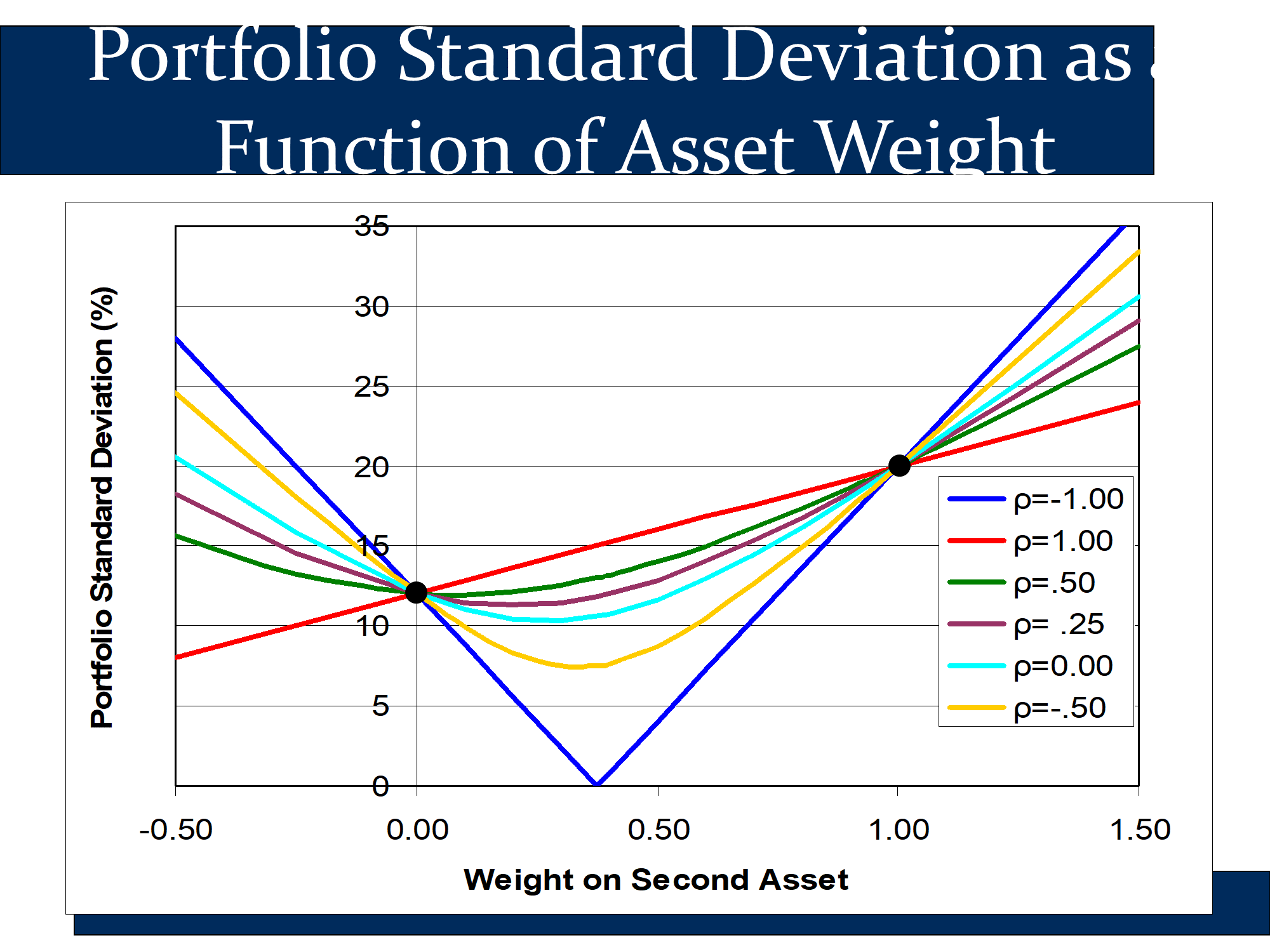
Whenever something has a negative correlation, think of it as insurance, because it cancels out risk. As you can see in the following slide, with a correlation of ρ=-1, you can actually cancel out all of your risk. You pay for this.

DON’T WORRY ABOUT A NEGATIVE BETA IN PROBLEMS. Our core CAPM formula will work for any value of beta, whether it is positive or negative. Therefore, we don’t need to worry

🙋 Can you compare and contrast systematic risk, idiosyncratic risk, total risk, and beta?

See answer

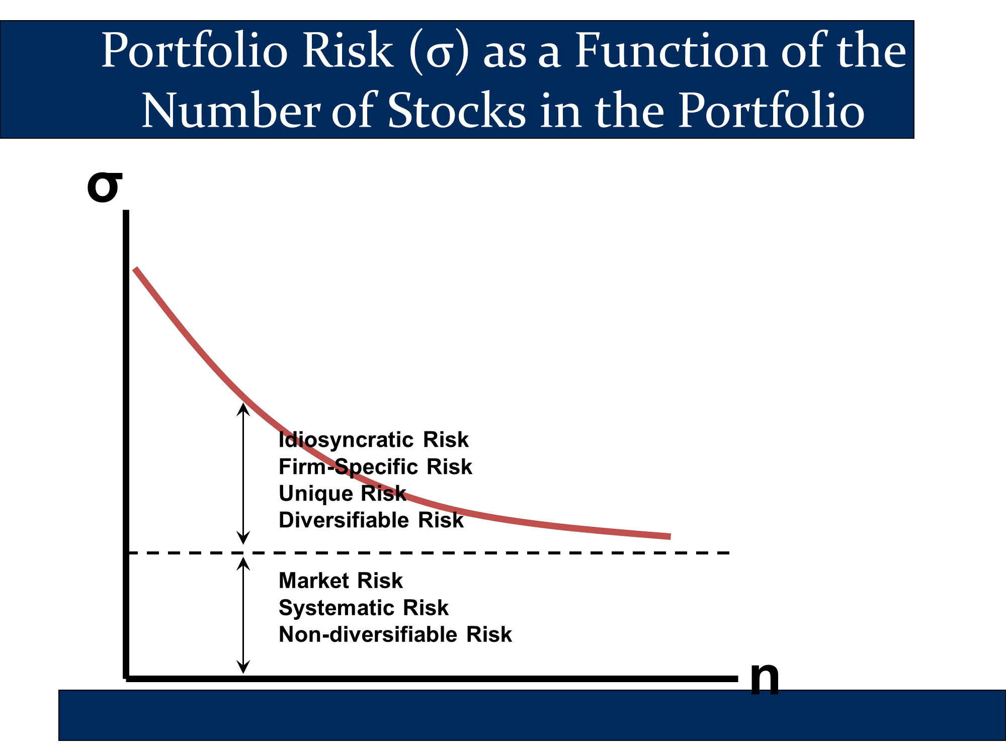
✔ Intuitively, σ = total risk = systematic risk + idiosyncratic risk
In other words, total risk can be broken down into a systematic component and an idiosyncratic component.

β is a measure of the systematic risk of a stock or portfolio. From the key equation of the CAPM, it follows that β is the only thing that determines securities prices:

$$E(r_i) = r_F + β(E(r_M)-r_F)$$

In other words, according to the CAPM, idiosyncratic risk does not affect securities prices at all.

🧠 Advanced: Let’s do an example to understand this a little more clearly. Suppose you run a hedge fund that is hedged against the overall return of the market, so its correlation with the market is exactly 0. (I’ll be happy to discuss how a long/short fund could accomplish this.) Because β is a measure of correlation with the market, this hedge fund will have a β of 0. As a result, investors will consider your hedge fund to have no market risk/systematic risk/non-diversifiable risk. Within the CAPM, each investor will hold a tiny portion of assets like your fund, and they will hold them in such a well-diversified portfolio that they are able to diversify all of the risk away. As a result, they will not demand any return from your fund. (Basically, each investor will hold such a small stake in your fund and in similar funds that all risk is diversified away.) This explains why hedge funds often loudly proclaim that they are a good source of “uncorrelated returns.” They are essentially bragging that their funds have a low beta. With a low beta, the risk from their fund can be essentially diversified away. With almost no non-diversifiable risk, investors don’t need to demand a high return: E(ri) = rF + β(E(rM)-rF) ≈ rF + 0(E(rM)-rF) = rF In this light, even if the hedge fund has even a very small or an unreliable return, with so little non-diversifiable risk, the hedge fund can command high management fees. 💲

🙋 in general when HPR < E(r) CAPM calculation, then the stock is underpriced? correct?

See answer

✔ Close, but the reverse of this.

The CAPM tells you what a fair return for the stock would be, given it’s beta. HPR (Holding Period Return) tells you the actual return that you think the stock will make. If the actual return is lower (ie HPR < CAPM E(r)) then the return is low because you paid too much for the security - ie it is overpriced.

If something is overpriced, you are paying too much, so the actual return you get (HPR) will be less than you should get based on its systematic risk (CAPM E(r)).
If something is underpriced, you are getting a good price, so the actual return you get (HPR) will be greater than you should get based on its systematic risk (CAPM E(r)). (think Warren Buffet - his goal is to get high HPRs by buying underpriced securities- ie value securities)
If something is correctly, the actual return you get (HPR) will be equal to the return you should get based on its systematic risk (CAPM E(r)).

✏️ Continuing the last problem, suppose that the actual market price of the stock is $90. Is it overpriced or underpriced?

✔ underpriced. If the stock is sufficiently underpriced / below its target, you should buy.

Another way to think about it is that if you know the future value of a stock, then:

• Anything with a return higher than you would expect has a high return because it is cheap (undervalued).
• Anything with a lower return than you would expect has a high return because it is expensive (overvalued).

Suppose a stock will be worth $10 in a year (you will receive a dividend of $1 and can sell it for $9). We can think about it as a “fixed income” instrument (ie a bond) in this case.

• When it’s current price goes down (relative to its future value), it’s return goes up.
• When it’s current price goes up, it’s return goes down.
  Just like a bond…

Based on its nondiversifiable risk it should have a return of 11.11%. If it had a price of $9 today, it would get that return.

With a price above $9, it is overpriced and will have a return less than 11.11%. (🧠: overpriced = low return).

With a price below $9, it is underpriced and will have a return higher than 11.11% (🧠: underpriced = high return).

Another way to approach the underpriced/overpriced question is to ask what the return is. If you know how much the stock is going to be worth next year and the current stock price leads to a return greater than CAPM would predict, it means that the current stock price is too low. Remember, lower prices always mean higher returns.

🙋 #8 what does he mean by the “Forecasted Return?” So should my answer be my new CAPM E(r) calculation… not the same forecasted return… ? Also, what does fair return mean?

See answer

✔ Forecasted return means the returns predicted by your analysts (not the CAPM).

Fair return means according to the CAPM: E(ri) = rf + β(E(rM)-rF)
Investors will demand a higher E(ri) for securities with a higher nonsystematic risk. Thus, a higher return is “fair” for securities with a higher nondiversifiable (ie systematic) risk.

🙋 When do we equal E(r) with HPR?

See answer

✔ We always equate expected HPR with E(r) You always equate r_i with HPR

HPR is just the Return that you get “during the Period you Hold the security.” In other words, it is the actual return you get. The CAPM predicts that your HPR will be rf + β(E(rM)-rF)

🙋 What is α?

See answer

✔ Intuitively α is “extra” returns you get as a result of your skills.

There is a website “seeking Alpha” for stock pickers. They are trying to outperform the market, and get “extra returns.”

Per the following diagram:

$$\begin{aligned} α &= E(r_i) - \text{the expected return from the CAPM} \\ &= \text{Expected-Return - Expected-Return-Based-On-Beta} \end{aligned}$$

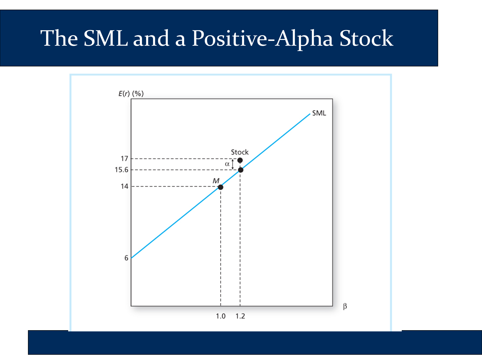
CAPM tells you the amount of return that is “fair” or that is demanded by the market based on the level of nondiversifiable risk. This fair return is E(r_i)=r_F + β(E(r_M)-r_F). If you can get some “extra” return, that is α.

Alpha is much more famous than beta.

If your analysts were perfect, they could estimate the probabilities of different returns the stock might earn.

Suppose Warren Buffet said, I’m going to flip a coin. If it comes up heads, I’ll give you $1M. Tails, nothing. I will charge you .5M to play. You hire analysts, they decide that the coin isn’t entirely fair and that the probability of heads is only 40%. They are wrong. The coin is fair, so if you had perfect analysts they would tell you that the probability of heads is 50%.

Their forecasted return for the bet will be less than the true expected return, E(r), for the bet.

According to CAPM, the perfect analysts say E(r) = …..

However, the CAPM is frequently wrong. Perfect analysts might say something different.

In the real world, we don’t know what perfect analysts would say. We only have the forecast from OUR analysts, which will likely differ from the CAPM forecast.

If our analysts predict a higher return than the CAPM, they are predicting a positive α>0

🙋 Where does the efficient frontier come from?

See answer

✔ The efficient frontier is what you get when you plot out the returns off all possible weightings of your N securities. You use the equations from class to plot this out.

But where do the input E(ri) and σi come from? 🙋‍♂️: “in particular which time period are they assessed from?”

If you want to use modern portfolio theory, then you will need to come up with E(ri) through very careful analysis. Hire a team of CFAs (Chartered Financial Analysts) to get E(ri). There are better techniques for assessing correlations, covariances, and variances from past data.

🙋 Where does β come from? Could we use 52 week high or low?

See answer

✔ There is a formula for beta that we I gave you in section. But you can use it to calculate Beta. If you’ve taken statistics, it corresponds to “Ordinary Least Squares regression.”

β = Cov(r_m, r_i)/(σ_m * σ_i)

= (σ_m * σ_i * p_12)/σ_m²

Yahoo Finance crunches the numbers for you.

🙋 Interpretation of Q6

See answer

✔ Risk premium is E(ri)-rf

Risk premium depends on β, because Risk premium = E(ri) - rf = β(E(rM)-rF) In other words, the risk premium of any stock is β × risk premium of the market.

How do the matrix versions of the Portfolio Variance formula work?

See answer

Full Question:
🙋 I have a question regarding slide 16:

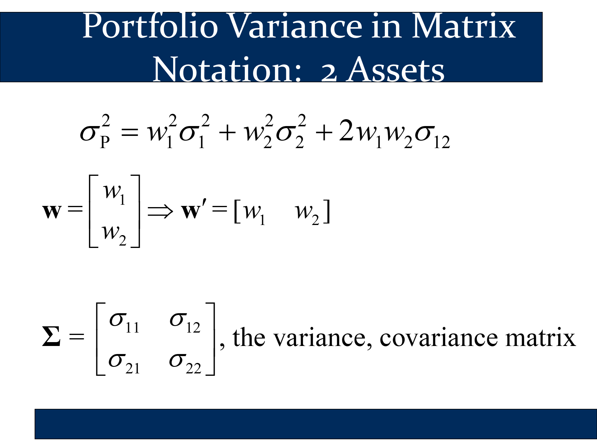
We have the inverse of w which is a 1x2 and Σ which is a 2x2 matrix so the outcome result will be 1x2. By doing the multiplication we get

[w1*σ11+w2*σ21 w1*σ12+w2*σ22]

How the above which is a matrix can represent a single variance figure according to the formula on top of the page?

✔ The actual formula you want is

$$\begin{aligned} σ_P^2 &= w' Σ w \\ &= \begin{bmatrix}w_1 & w_2 \end{bmatrix} \begin{bmatrix} σ_{11} & σ_{12} \\ σ_{21} & σ_{22} \end{bmatrix} \begin{bmatrix}w_1 \\ w_2\end{bmatrix} \\ &= \left(\begin{bmatrix}w_1 & w_2 \end{bmatrix} \begin{bmatrix} σ_{11} & σ_{12} \\ σ_{21} & σ_{22} \end{bmatrix} \right) \begin{bmatrix}w_1 \\ w_2\end{bmatrix} \\ &= \left( \begin{bmatrix} w_1σ_{11} + w_2σ_{21} & w_1σ_{12} + w_2σ_{22} \end{bmatrix} \right) \begin{bmatrix}w_1 \\ w_2\end{bmatrix} \\ &= (w_1σ_{11} + w_2σ_{21})w_1 + (w_1σ_{12} + w_2σ_{22})w_2 \\ &= w_1σ_{11}w_1 + w_2σ_{21}w_1 + w_1σ_{12}w_2 + w_2σ_{22}w_2 \end{aligned}$$

[Note that the covariance between a variable and itself is just the variance of that variable. Therefore, $σ_{11} = σ_1^2$ and $σ_{22} = σ_2^2$ . Likewise there is a math fact that says that $σ_{21}=σ_{12}$. Substitute in, we get:]

$$\begin{aligned} σ_P^2 &= w_1σ_1^2w_1 + w_2σ_{12}w_1 + w_1σ_{12}w_2 + w_2σ_2^2w_2 \\ &= w_1^2σ_1^2 + w_2^2σ_2^2 + w_1σ_{12}w_2 + w_1σ_{12}w_2 \\ &= w_1^2σ_1^2 + w_2^2σ_2^2 + 2w_1w_2σ_{12} \\ \end{aligned}$$

The above is just the “classic formula from probability” for variance.