🔎 Big Picture for Risky Portfolios

Just like last week, investment is a tradeoff between risk and return.

Therefore, just like in last week, your eye out for the formulas for expected return and standard deviation.

Last week, they were for the “complete portfolio”:

$$E(r_C) = r_F + y(E(r_P) - r_F)$$

      or $E(r_c) = yE(r_P) + (1-y)E(r_F)$

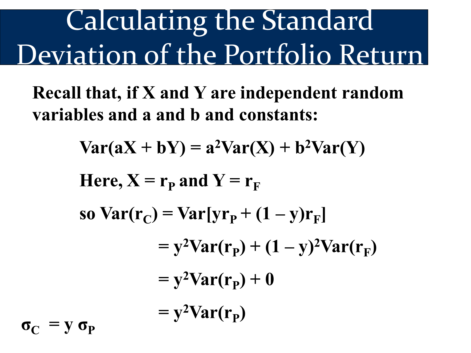
$$σ_C = yσ_P$$

Now, we have equations for combing two risky assets into a optimal risky portfolio:

$$E(r_p)= w_1 E(r_1) + w_2 E(r_2)$$ $$σp = SQRT(σ_1^2 w_1^2 + σ_2^2 w_2^2 + 2w_1 w_2 Cov_(1,2))$$

Optimal Risky Portfolios & CAPM

Name	Equation
Expected Return of 2+ risky assets	$E(r_p) = (Er_1 \times w_1) + (Er_2 \times w_2)$ …
If you have a target for $E(r_P$)	$w_1 = \frac{(E(r_p) - E(r_2))}{(E(r_1) - E(r_2))}$ → $w_2 = 1 - w_1$
Standard Deviation 2 risky assets	$σ_p = SQRT(σ_1^2 w_1^2 + σ_2^2 w_2^2 + 2w_1 w_2 Cov_{(1,2)})$ $σ_p = SQRT(σ_1^2 w_1^2 + σ_2^2 w_2^2 + 2w_1 w_2 σ_1 σ_2 ρ_{(1,2)})$
Standard Deviation 2 risky assets (Spreadsheet-friendly formula)	$σ_p = SQRT((σ_1^2 \times w_1^2) +(σ_2^2 \times w_2^2)+(2 \times w_1 \times w_2 \times Cov_{(1,2)})$ $σ_p = SQRT((σ_1^2 \times w_1^2) + (σ_2^2 \times w_2^2) + (2 \times w_1 \times w_2 \times σ_1 \times σ_2 \times ρ_{(1,2)}))$
Standard Deviation 3 risky assets	$= SQRT((σ_1^2 \times w_1^2) + (σ_2^2 \times w_2^2) + (σ_3^2 \times w_3^2) +$   $(2 \times w1 \times w2 \times Cov_{(1,2)}$ + $(2 \times w_1 \times w_3 \times Cov_{(1,3)}) + (2 \times w_2 \times w_3 \times Cov_{(2,3)}))$
Covariance $(r_1,r_2)$	= $E[(r_1-Er_1) \times (r_2-Er_2)]$
Correlation Coefficient $(ρ_{1,2})$	$ρ_{1,2} = \frac({Cov_{r_1,r2})}{(σ_1 \times σ_2)}$ → (ρ is between -1 and 1) $Cov_{(r_1,r_2)} = σ_1 \times σ_2 \times ρ_{1,2}$
Utility Function	$U=E(r)-\frac{1}{2}Aσ^2$
Capital Asset Pricing Model $(CAPM)$	$Er_P = r_F + (B \times (Er_M-r_F))$

$w_1$ = portion invested in asset 1 $w_2 = (1-w_1)$ = portion invested in asset 2 $E$ = expected $r$ = return for asset $σ$ = Standard Deviation

$ρ_{1,2}$ = correlation between assets 1 and 2 $p$ = portfolio $r_F$ = risk-free rate $β$ = Beta