🔎 CAL vs CML vs SML

Executive Summary

The CAL is what we covered two weeks ago. It shows the relationship between $σ$ and $E(r_c)$ .
The CML is just the CAL the CAPM says people will construct. It is the CAL constructed when using the market portfolio as the risky portfolio.
- The market portfolio is a portfolio that contains all possible risky investments. It holds each investment in proportion to its market cap. In the CAPM everyone chooses the market portfolio as their risky portfolio.
The SML is different. Rather than showing the relationship between $σ$ and $E(r)$ , it shows the relationship between $β$ and $E(r)$ . it is a plot of the main CAPM equation: $E(r_s) = r_f - β(E(r_m) - r_f)$

Starting with the lecture on the CAL, we did a three lecture sequence. The first two lectures introduced “Markowitz Portfolio Optimization,” which is summarized in my spreadsheet from the previous lecture. The final week was the CAPM. Rather than telling you how to optimize your own portfolio, CAPM is a model of how the entire investment market works — in other words it is a “Capital Asset Pricing Model.” To derive its conclusions it assumes that all investors use Markowitz Portfolio Optimization. That is why we cover Markowitz Portfolio optimization before the CAPM.

The CAL - Capital Allocation Line

The CAL is part of Markowitz Portfolio Optimization. The CAL is you “menu of options” whenever you combine a risky portfolio and a risk-free asset.

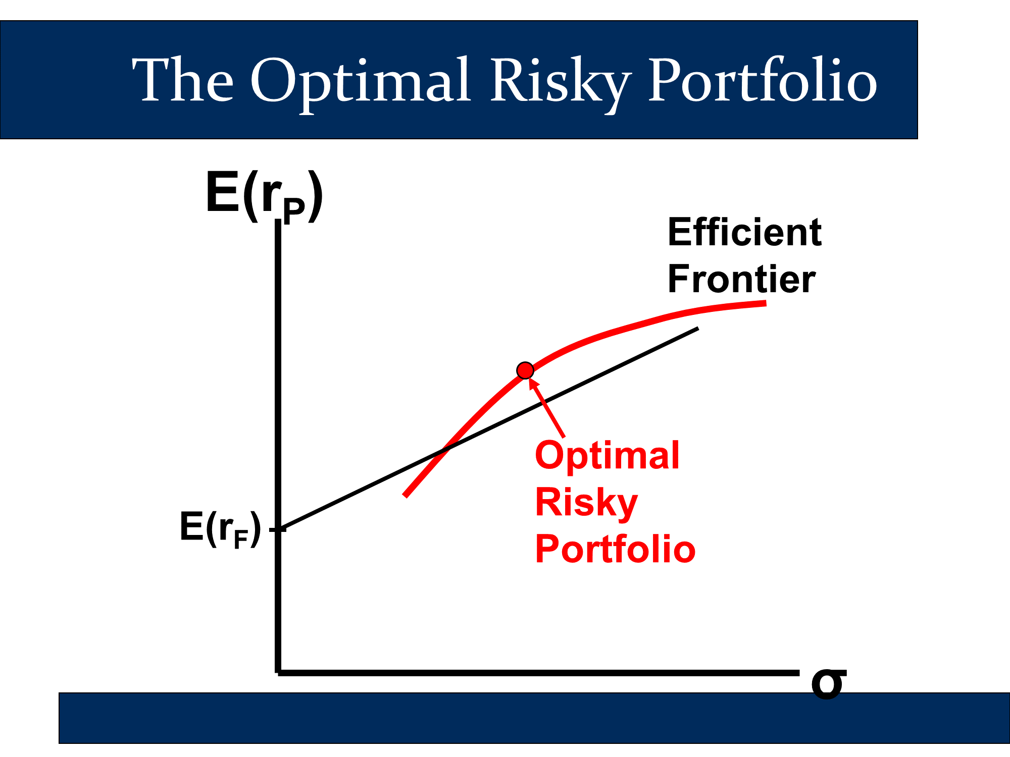
Steps in Markowitz Portfolio Optimization

Step 1: Find the optimal risky portfolio
Step 2: Make a CAL using the optimal risky portfolio
Step 3: Based on your indifference curves, choose an optimal complete portfolio from the CAL.

These steps are illustrated in my spreadsheet: https://robmunger.com/1920mpt

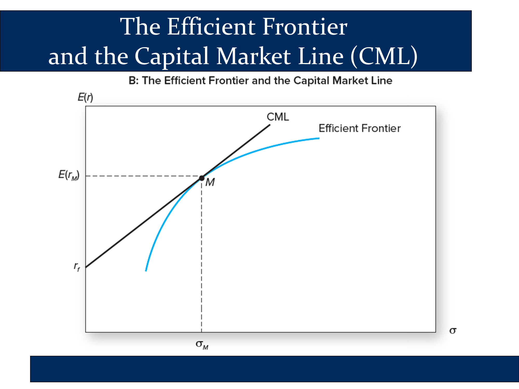
The CML - Capital Market Line

The CML may look like the CAL, but it isn’t part of a typical Markowitz Portfolio Optimization. Rather, it is part of the CAPM.

You can think of the CAPM as being like a computer simulation in which all of the simulated people are using Markowitz Portfolio Optimization to choose their investment portfolio. The simulation assumes that people use Markowitz because the simulation needs to assume something and Markowitz provides concrete steps to simulate. The simulation then uses the logic of supply and demand to determine prices and returns for all possible securities. Wow!

Whereas Markowitz Portfolio Optimization is a concrete technique for choosing a portfolio, the CAPM is a “big think” way of concentrating the entire securities market.

Illustration below… (image credit: Reddit user “Ursson”) ⇩

In the CAPM’s simulation, all of the simulated people find the same optimal risky portfolio. This is because they all use the same assumptions about future value of the securities. The optimal portfolio they come up with is the portfolio of all available investable assets, weighted by their market capitalizations (this is equivalent to saying that they all buy index fund). We call this “uber index fund” optimal risky portfolio “the market portfolio.” In Markowitz optimization, the next step is to find the Capital Allocation Line, so everyone in the CAPM model does this next. The CAL that they come up with is called the Capital Market Line.

🙋‍♂️In the CAPM Sim City simulation, is everyone identical, except for their indifference curves/risk aversion?

See answer

Yes. They use the exact same inputs about future security values and they follow exactly the same analysis (Markowitz). We make these assumptions because they “aren’t terrible” and they allow us to draw conclusions.

Therefore, the CML is a special name for the CAL in the CAPM. It is unique because in the CAPM, everyone chooses the market portfolio as the risky portfolio. It sounds like it is part of Markowitz, but it is actually part of the CAPM.

CAL vs CML

The CML is just the CAL, using the market portfolio as the risky portfolio. In other words, it is just the CAL as applied to the CAPM.

Remember, behind the CAPM are about 10-20 pages of calculations that we shield you from. Within those calculations, the individual investors in the CAPM are modeled as following the full process of Markowitz Portfolio Optimization/Modern Portfolio Theory that we covered during the last several lectures.
(This illustrates the idea that the CAPM is a complex mathematical model, akin to a simulation, and the formulas that we see are just some of the final steps in that model. It also illustrates the rationality assumptions that are used to build the model (because the investors are rational, then they must use Markowitz Portfolio Optimization, as it is the mathematically optimal way to optimize a mean-variance portfolio (several other of the assumptions of the model are required to conclude this).))

Markowitz Portfolio Optimization can be done with any list of stocks. The CAPM is a specific simulated application of Markowitz. In it, all of “the little sims” do Markowitz with the same inputs and get the market portfolio.

If you used the same inputs as them and did Markowitz, you would get the CML as your CAL.

How to calculate the slope if the SML

Let’s calculate the Expected return at $β=0$ and $β=1$ .

$x=β$	$y=E(rS)$
$0$	$E(r_s)=r_f + β(E(r_M)-r_f)$ $=r_f + 0(E(r_M)-r_f)$ $=r_f$
$1$	$E(r_s)=r_f + β(E(r_M)-r_f)$ $=r_f + 1(E(rM)-r_f)$ $=r_f + E(r_M)-r_f$ $=E(r_M)$

Slope = rise/run

rise = $Δy = E(r_M) - r_f$ ← taking the values from the 2nd column of the table.
run = $Δx = 1-0 = 1$ ← taking the values from the first column of the table.

The SML - Securities Market Line

I expressed amazement above that the CAPM can simulate a price and return for all possible securities. That’s pretty amazing if you think about it.

All it needs to forecast the expected future return, $E(r_s)$ , is the security’s beta, $β_s$ , which can be calculated from past daily returns.

In other words, the CAPM predicts the required return for any security based only on that security’s statistical β. This is worth graphing.

Literally, all the SML is is a graph of $E(r_S)=r_f+β(E(r_M)-r_f)$

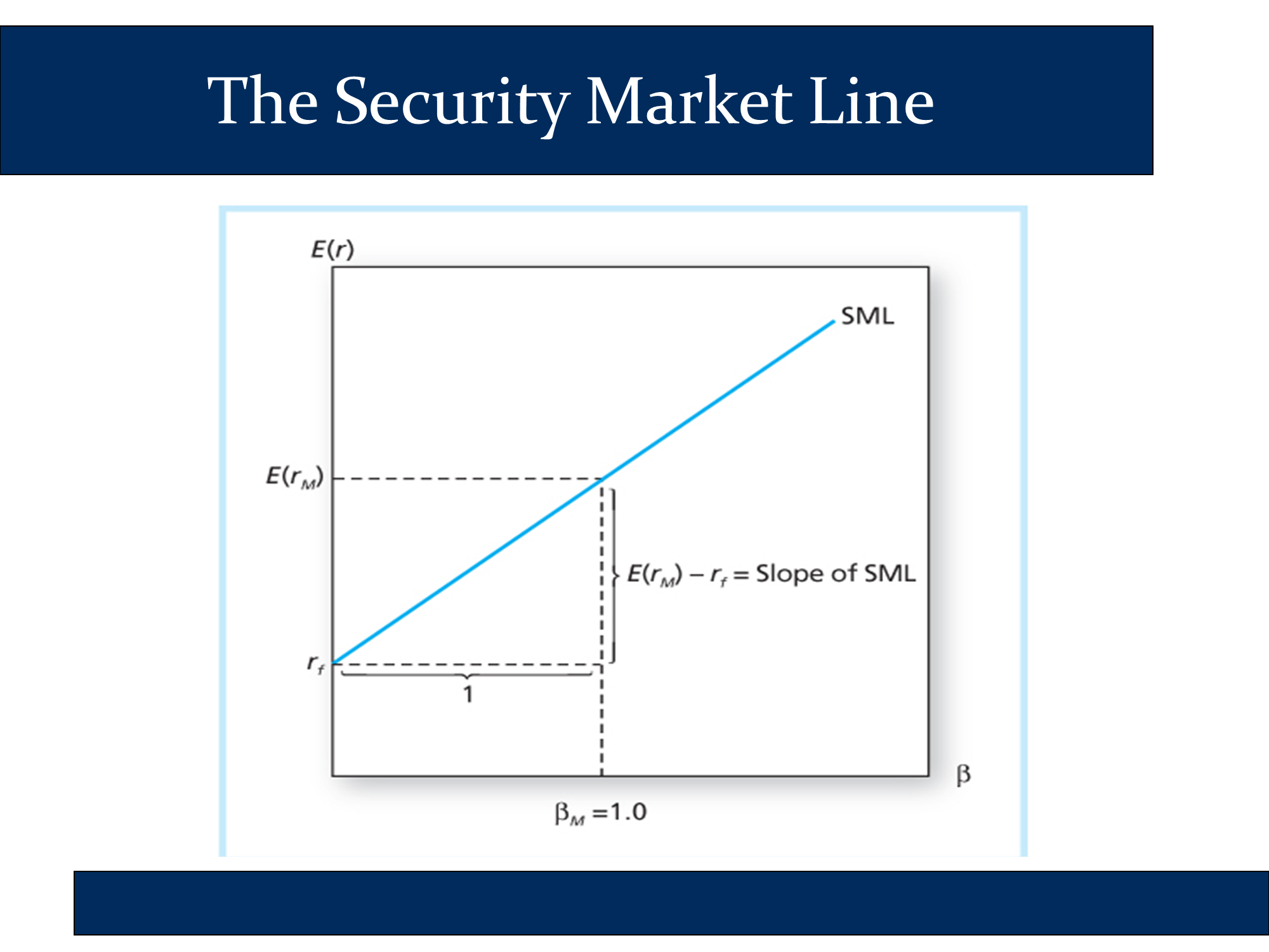
Takeaways: the SML is just the graph of $E(r_S)=r_f+β(E(r_M )-r_f)$

In fact, you could call that equation the “SML” because it tells you the returns on different securities in the market, based on the CAPM.

The SML predicts the expected return for any security (15.6% in the diagram below).

If you expect a security to have a higher return (say 17%), that is equivalent to saying the security is expected to “outperform” by $17\%-15.6\%=1.4\%$ . We call this outperformance $α$ .

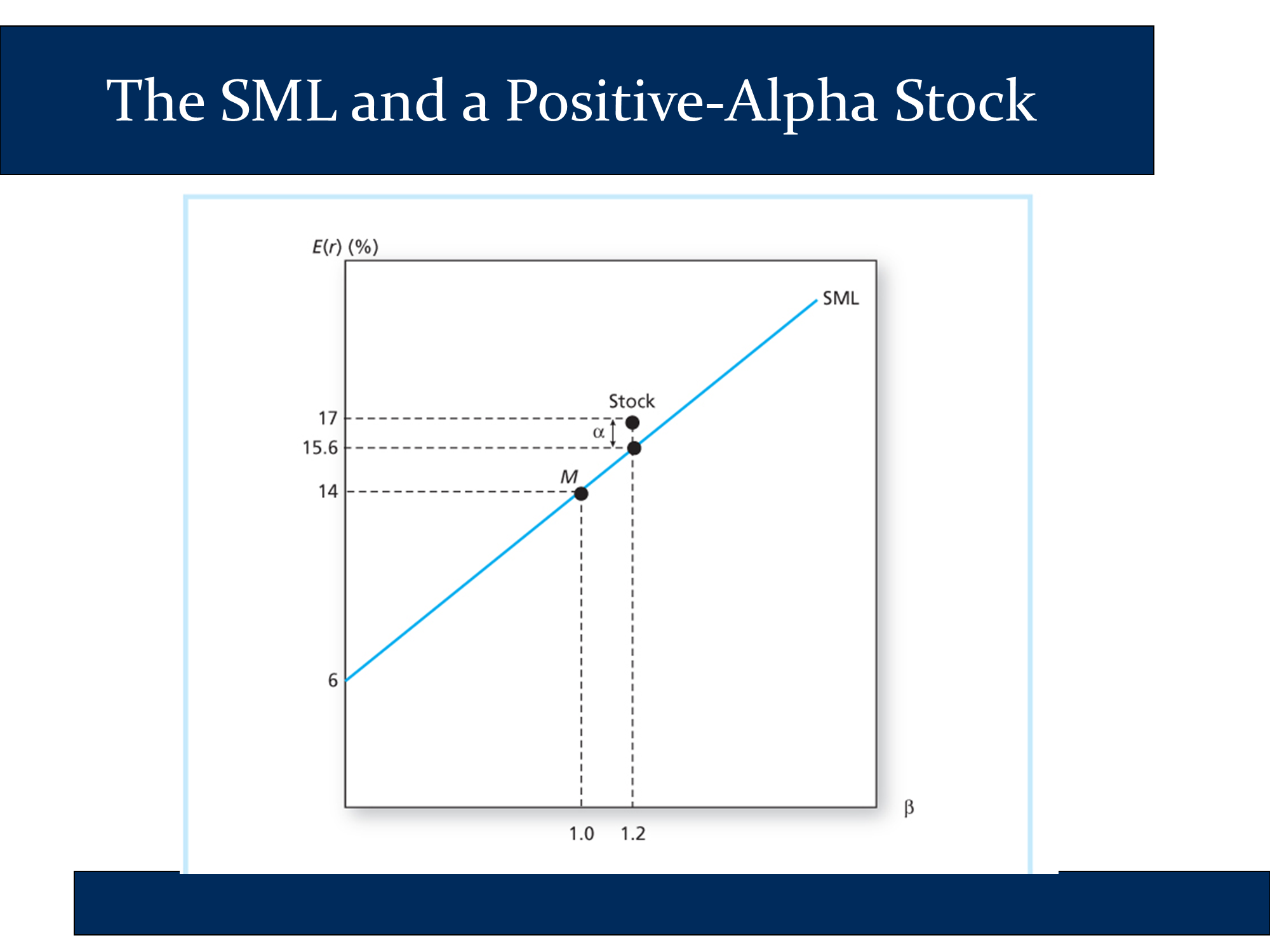
If $α>0$ , “you should buy” and “the stock is underpriced”
If $α=0$ , “the stock is fairly priced”
If $α<0$ , “you should sell” and “the stock is overpriced”

Summary

In summary,

The CAL shows all mixtures of a risk free asset and a risky portfolio.
When the risky portfolio is the “market portfolio,” we refer to the CAL as the CML.
The SML is just a graph of $E(r_S)=r_f+β(E(r_M)-r_f)$

The diagrams differ based on what is on the x-axis.

the CAL and CML show the relationship between σ and Er based on mixtures of risky and risk-free assets.

Therefore, σ is on the x axis.
the SML shows the relationship between β and Er based on the CAPM.
Therefore, β is on the x axis.