🔎 Quick duration calculations
This page will show you how to quickly create a table to calculate Duration for a bond in Excel.
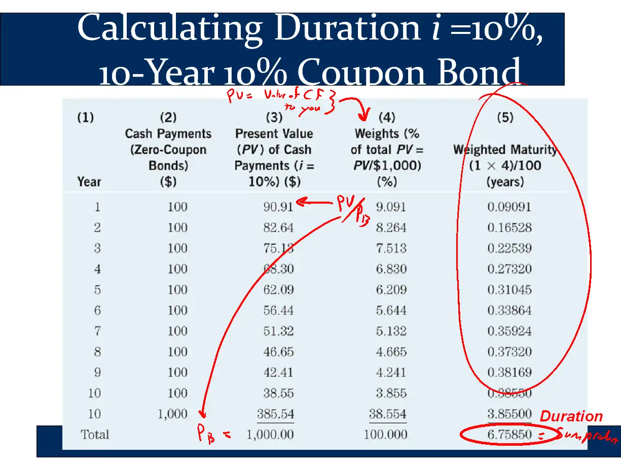
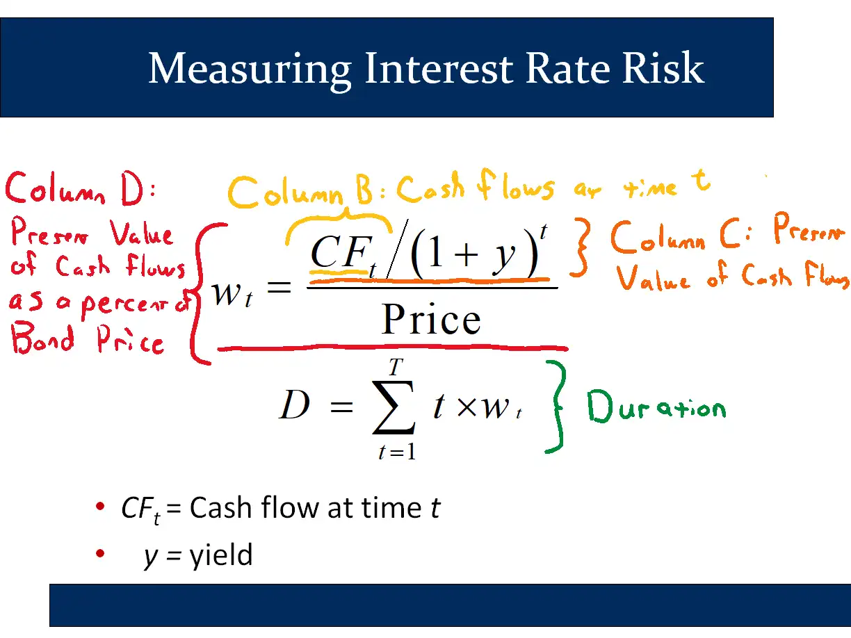
It implements the table on the following slide from Bruce’s presentation:
If you study it, you will be able to make a table like the following, starting from a blank worksheet, in under 2-3 minutes. You don’t need to know anything or own any software as there are free alternatives. (Note: Don’t read it using mobile data - wait until you have a wifi connection, as there are some moderately large files in this page.)
You will learn several very valuable spreadsheet skills that will work in Excel or Google Sheets (free). [incidentally, my very impressive IT wife was looking over my shoulder when I was making this and exclaimed, “HOW DO YOU MAKE IT DO THAT!!!” See below to find learn this valuable Excel skill!] Remember, you can always shoot me an email if you are stuck.
I will assume that you know the very basics of spreadsheets in this page. If you don’t, please watch a tutorial for beginners such as this one for Excel or the first third of this one for Google Sheets. (Google Sheets is free and just as capable as Excel.)
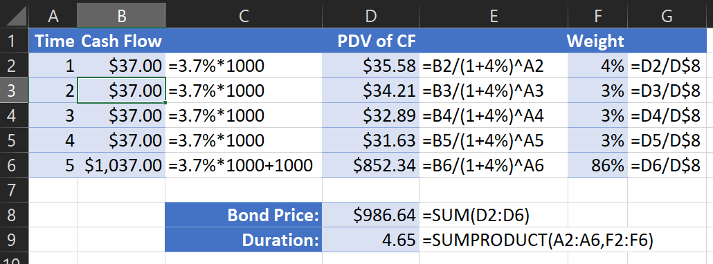
Step 1: Fill in row 1 and columns A and B from the example table above.
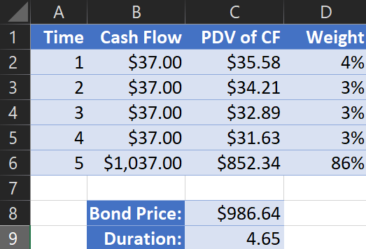
The example above is based on a bond with the following characteristics:
Maturity: 5 years
Coupon Rate: 3.7% (annual coupons)
Yield to Maturity: 4%
Face Value: $1000
(For a duration question, the Face value doesn’t matter. If you aren’t told the face value, just assume F=$100 or F=$1000.)
For this step and the next two steps, be sure to use your spreadsheet’s amazing autofill function by grabbing the tiny little square that appears when you select cells. Your pointer will turn into a bold black plus-sign when you hover over the square. (Watch below for an example.)
Watch the quick video here for an overview:
Or watch me demonstrate it:
Step 2: Find the Present Discounted Value of each Cash Flow (Column C) and sum them to get the bond price.
The formulas for column C will be as follows:
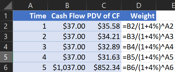
In the above, ‘B2’ refers to the number in the column B and row 2. Likewise ‘A2’ refers to column A and row 2. If you aren’t familiar with this idea, known as cell references, be sure to watch the following video: Understand and Use Cell References. (This video applies to all versions of all spreadsheets, not just Excel 2013)
As in step 1, you can greatly accelerate the process by using autofill. If you have put the formulas in using cell references, like I did above, your spreadsheet will automatically put the numbers in correctly:

Some notes on the above demonstration:
- To rapidly enter the cell references, I just clicked on cells I wanted to refer to (B2 and A2 for the first line). To learn more, watch the “Understand and Use Cell References” video mentioned above. It’s a great video and a valuable skill!
- I used “ShowFormula” to show the formulas, but you can skip that step.
- To calculate the bond’s price, I just summed up each of the PDVs. This was made much easier by - you guessed it - cell references. You can watch that that same Understand and Use Cell References video to see a demonstration of adding numbers up with cell references. (Seriously, do this and thank me later. It will be the most valuable 2 minutes of your whole day. [email me if I’m wrong!])
Step 3: Calculate the weights (Column D) and duration
Column D is the duration weights. These are just the PDV of the cash flows from that time period (ie that row) divided by the price of the bond. The following slide shows that this is exactly what we need to calculate the duration weights:
To calculate it rapidly, we use autofill and cell references, as above.
In step 2, when we did autofill, Excel automatically adjusted cell references when you did autofill. However, we don’t want it to do this to the bond price. Therefore, in the following video, rather than dividing by ‘C8,’ I divide by $C$8. This “locks” the reference onto the bond price.
Once you’ve done that, use the weights to calculate duration. This is done most easily using the “SumProduct” function, selecting the time column, pressing comma, and selecting the weights column. This will calculate the weighted average of the times, using the given weights. (Sumproduct is also very helpful for calculating expected values and standard deviations.)
Technically speaking, using a dollar sign to lock a cell reference is known as “using an absolute rather than a relative cell reference.” It’s also a valuable skill to learn, but less important for duration because you only need to remember to do it once. However, if you want to learn more and get more practice with cell references, click here to find a tutorial that will also give you a bit of practice with cell references in general to boost your confidence.
Practicing and Checking Your Work
Okay, now it’s your turn. Try to do each of the steps on your own in your spreadsheet of choice. The following screenshot shows the formulas used for each column and cell.
Once you’ve done it once, try it again. And then again. I just timed myself and I was able to do it in a minute and 15 seconds, but I don’t have to refer to any lists or anything like that. Please let me know how it goes!